Counting trucks from space with free satellite data

1. Where the pictures come from

Everything here is built on one source of data: Sentinel-2, a set of three Earth-observation satellites run by the European Space Agency (ESA) as part of the European Union’s Copernicus programme.

If you’ve never heard of it, here is the whole thing in a paragraph. Copernicus is the EU’s flagship Earth-observation programme, and it is enormous: the European Union and ESA have poured well over €10 billion into it. Its guiding principle is unusual for something that expensive — the data is free and open to everyone, no login, no licence, no fee, from the very first image. A farmer in Hungary, a climate scientist in Chile, a hobbyist with a laptop, and a multinational all get the same pixels on the same terms. This project is a small demonstration of what that policy makes possible.

The Sentinel-2 satellites carry a single instrument, the MultiSpectral Instrument (MSI). Think of it as a very good digital camera that photographs the Earth in 13 separate colours (“bands”) instead of the three your phone uses — including bands your eye can’t see, like near-infrared. A few facts worth knowing:

Three satellites. Sentinel-2A launched in 2015, Sentinel-2B in 2017, and Sentinel-2C in 2024, all flying the same orbit on opposite sides of the planet. The archive now runs back a full decade.
The whole planet, every few days. The satellites image the entire land surface of the Earth — not just Europe. Any given spot is re-photographed roughly every five days at the equator, and more often toward the poles as the orbital tracks overlap, so a mid-latitude region like central Europe gets a fresh (cloud-permitting) look every 2–3 days.
A sun-synchronous orbit at ~786 km altitude means each spot is always imaged at roughly the same local time — about 10:30 in the morning. Over Hungary that works out to a snapshot at roughly noon local time. (This detail matters later.)
Free surface reflectance. The version we use (“Level-2A”) has already been corrected for the atmosphere, so each pixel is a physical measurement of how reflective the ground is — not just a pretty picture.
10-metre pixels in the visible and near-infrared bands. Each pixel covers a 10 m × 10 m square of ground — 100 square metres.

That last number is the hero and the villain of this whole story.

2. The catch: you cannot see a truck

Ten metres per pixel is astonishing for a free, whole-planet, every-few-days camera. It is also hopeless for looking at vehicles.

A lorry is about 2.5 m wide and 15–18 m long. That is smaller than a single Sentinel-2 pixel. A truck doesn’t fill a pixel; it tints one or two pixels slightly. There is no shape, no cab, no trailer — just a faint smudge that could be a truck, a bright roof, a road marking, or noise. If you crop the imagery down to the road and zoom in until the pixels are the size of dice, you still can’t point at a truck and say “there’s a truck.”

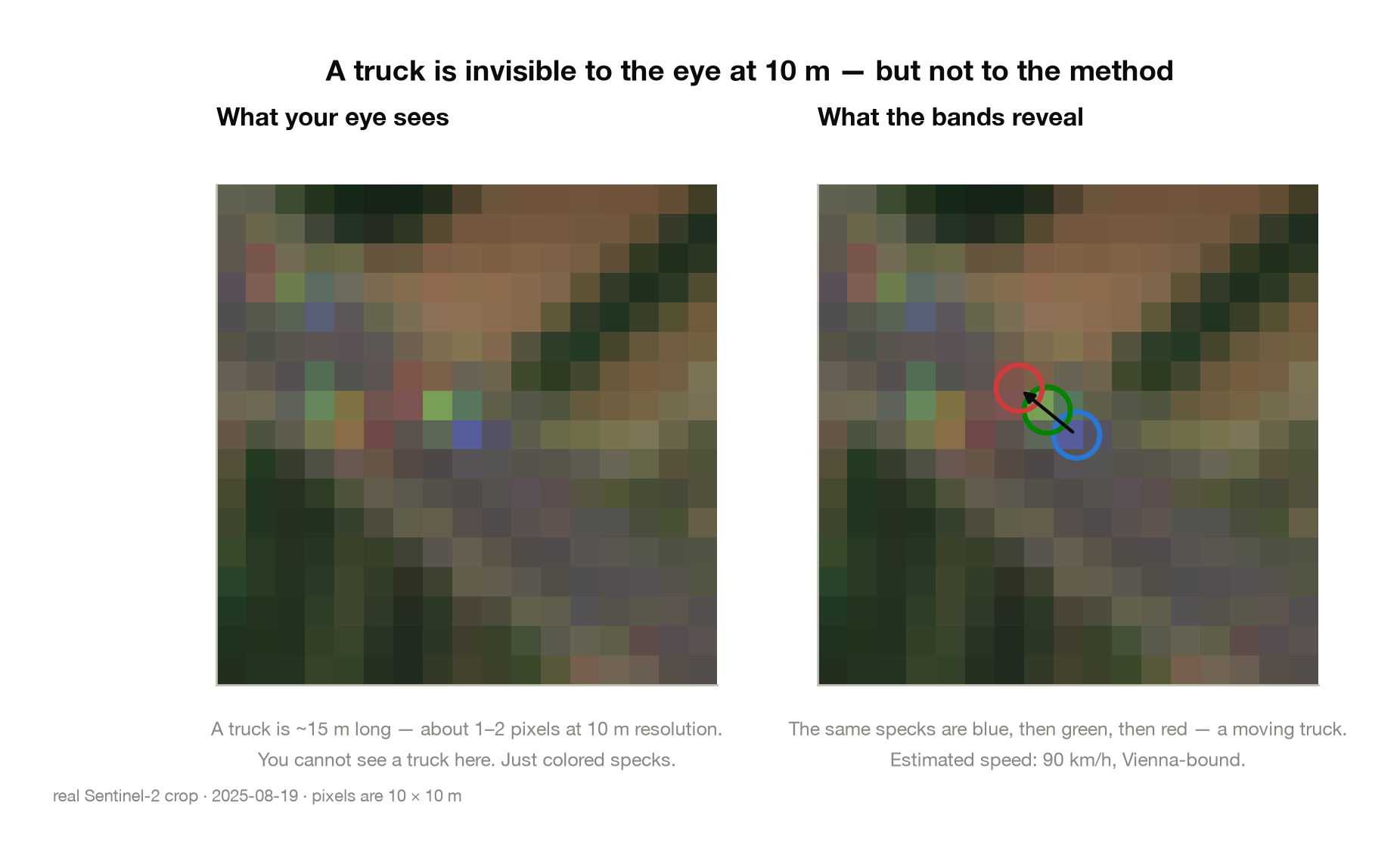
A truck is invisible to the eye at 10 m, but not to the method — Left: a real Sentinel-2 crop of the motorway. Somewhere in those coloured specks is a moving lorry — good luck spotting it. Right: the same pixels, decoded by the method in the next section.

So how do you count something you fundamentally cannot see? You stop trying to see the truck, and start looking for the trace it leaves in time.

3. The trick: moving things leave a rainbow

This is the clever part, and it is not my idea. The method was developed and published by Henrik Fisser and colleagues at the University of Würzburg — “Detecting Moving Trucks on Roads Using Sentinel-2 Data” (Fisser, Khorsandi, Wegmann & Baier, Remote Sensing, 2022). The underlying physics for measuring the velocity of moving objects from these same band offsets was worked out earlier by Henrik Heiselberg for ships and aircraft (Sensors, 2019). All the credit for the idea belongs to them; my contribution is only a clean re-implementation and the Budapest–Vienna analysis.

Here is the insight.

That “single photo” from Sentinel-2 is not actually taken all at once — and the reason is physical. The camera has no shutter that grabs a whole frame. Instead, each colour is recorded by its own separate row of detectors, each row sitting behind its own colour filter, and those rows are lined up one behind the next across the sensor. The satellite is a push-broom scanner, racing along its orbit at about 7 kilometres per second, so the ground streams past beneath it. A point on the road slides under the blue row first; then, a fraction of a second later once the satellite has moved on, under the green row; and later still under the red row. The colours are separated in time for the simple reason that the detectors are separated in space — they are different strips of silicon, and the satellite has travelled between them.

Concretely, green is captured about half a second after blue, and red about a second after blue. For anything standing still — a field, a building, the road itself — this makes no difference; it’s in the same place in all three exposures, so the colours line up perfectly.

But a truck doing 90 km/h travels 25 metres in one second — two and a half pixels. By the time the red detector looks, the truck has moved on. So the truck appears in three slightly different places, once in each colour, leaving a little blue → green → red streak pointing in its direction of travel:

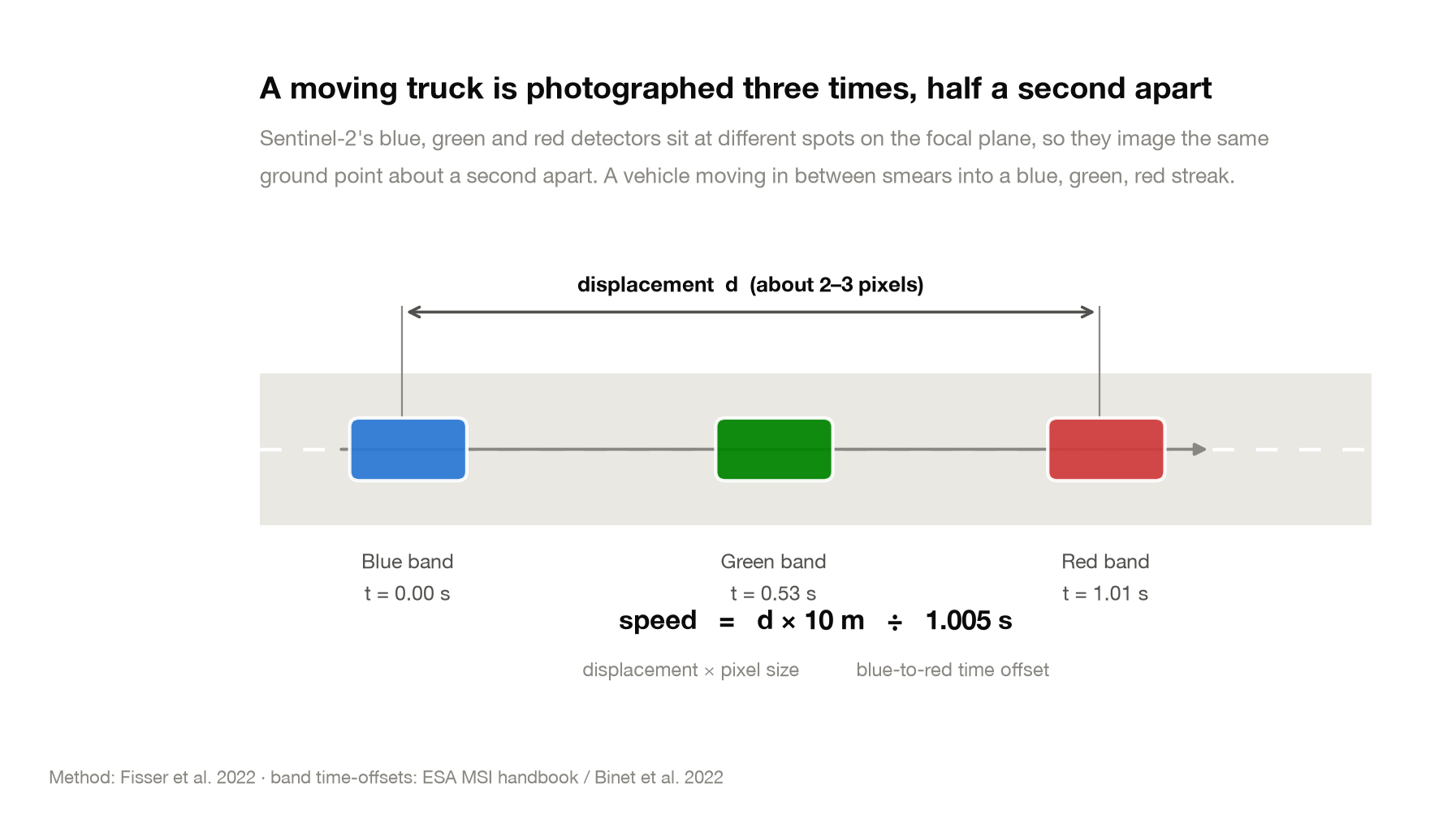
That streak is the fingerprint of motion, and it’s why a stationary bright object (which shows up in all three colours at the same spot, appearing white or grey) can be told apart from a moving one. Better still, the streak is a measurement. We know exactly how much time passes between the blue and red exposures — about 1.005 seconds (published in ESA’s instrument handbook and refined by Binet et al., 2022). Measure how far the truck moved between the blue and red positions, multiply by the 10-metre pixel size, divide by that time, and you have its speed. The direction of the streak, snapped to the direction of the road, tells you which way it’s going.

That’s the whole idea: a truck you can’t see, moving fast enough to paint itself across three colours, becomes a speed and a heading.

4. From rainbow to numbers: the implementation

Knowing the trick is one thing; running it over a year of a 240-kilometre motorway is another. The pipeline is five stages, each a small Python script, each writing its results to disk so the whole thing is restartable. (The full code is in the project repository.)

Stage 1 — Get the imagery (backfill_route.py). The images live in a public Amazon S3 bucket (sentinel-cogs) as cloud-optimised GeoTIFFs, indexed by a free STAC search API from Element 84. No account, no key. The nice property of cloud-optimised files is that you can download just the rectangle you care about over the network, instead of a whole 110 km × 110 km tile. So the pipeline: figures out which satellite tiles cover the Budapest–Vienna route, splits the route into small on-corridor boxes, and pulls only the four bands it needs (blue, green, red, and a “scene classification” quality band) clipped to those boxes — downloading in parallel to keep it quick. A year of the whole corridor comes to a few gigabytes instead of terabytes.

Stage 2 — Clean up (preprocess.py). Two jobs. First, throw away clouds: Sentinel-2 ships a per-pixel classification band, so we mask out anything flagged as cloud, cloud shadow, cirrus or snow, and record how much of the road corridor was actually usable in each scene. Second, focus on the road: we pull the exact geometry of the M1 and A4 motorways from OpenStreetMap, buffer it by 40 m, and keep only pixels on the carriageway. This one geometric filter removes almost every possible false positive — fields, water, rooftops — before detection even starts.

Stage 3 — Detect the trucks (trucks.py). On each cleaned, road-only scene we apply Fisser’s test for a “blue-leading” pixel (one where blue clearly dominates green and red — the front of the streak), group neighbouring hits into candidate trucks, then look nearby for the matching green and red positions. From the three positions we project the motion onto the road and read off speed and direction, keeping only physically plausible results (40–130 km/h, moving along the road, not across it). Every surviving detection is saved with a little image chip marking its three coloured ghosts — so any claim can be checked against the actual pixels.

Stage 4 & 5 — Aggregate and visualise (analyze.py, figures.py). Counts by direction, speeds, and the charts you’ll see below.

Two details caused real trouble and are worth flagging for anyone rebuilding this:

The reflectance offset. Recent Sentinel-2 files store reflectance with a hidden +1000 offset that you’re supposed to subtract — except the particular cloud-optimised files we read don’t actually carry it. Applying the “correct” formula turned 91% of the land negative. The fix (verified against the pixels) is to just divide the raw value by 10,000. A reminder that you should always look at your data, not just trust the documentation.
The direction ambiguity. Because of how the camera’s detectors are arranged, the raw blue→red direction can flip depending on which strip of the image a truck falls in. So we never trust the raw streak direction alone — we snap it to the known orientation of the road, which resolves it cleanly.

5. What a year of trucks looks like

Run over a year of clear-sky Sentinel-2 passes along the whole Budapest–Vienna corridor, the pipeline finds more than 17,000 individual moving trucks — each one a tiny rainbow smear, each with a position, a heading, and a speed. Pooled together, they draw a surprisingly detailed portrait of European freight.

Speed: a motorway with a slow spot

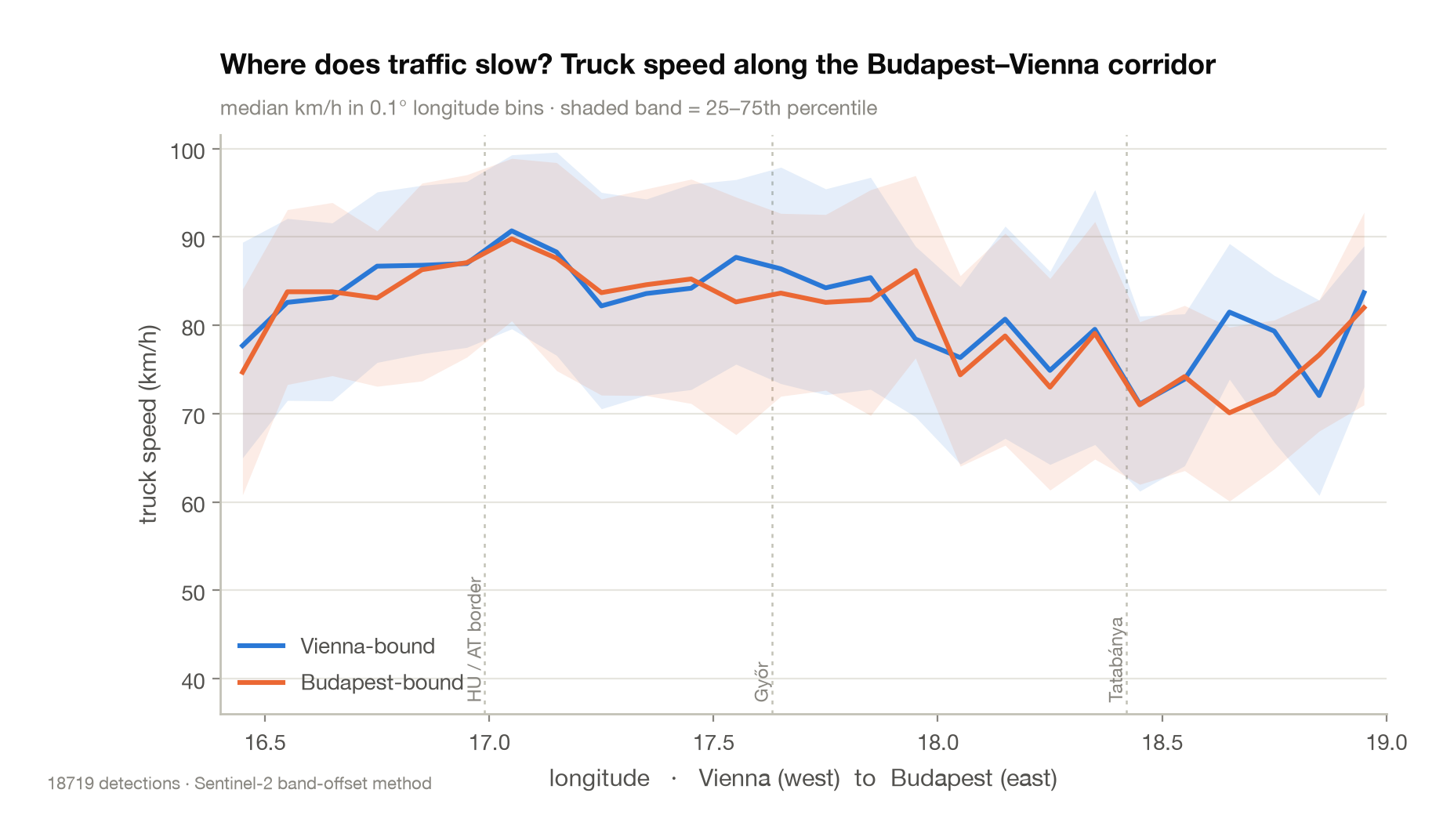
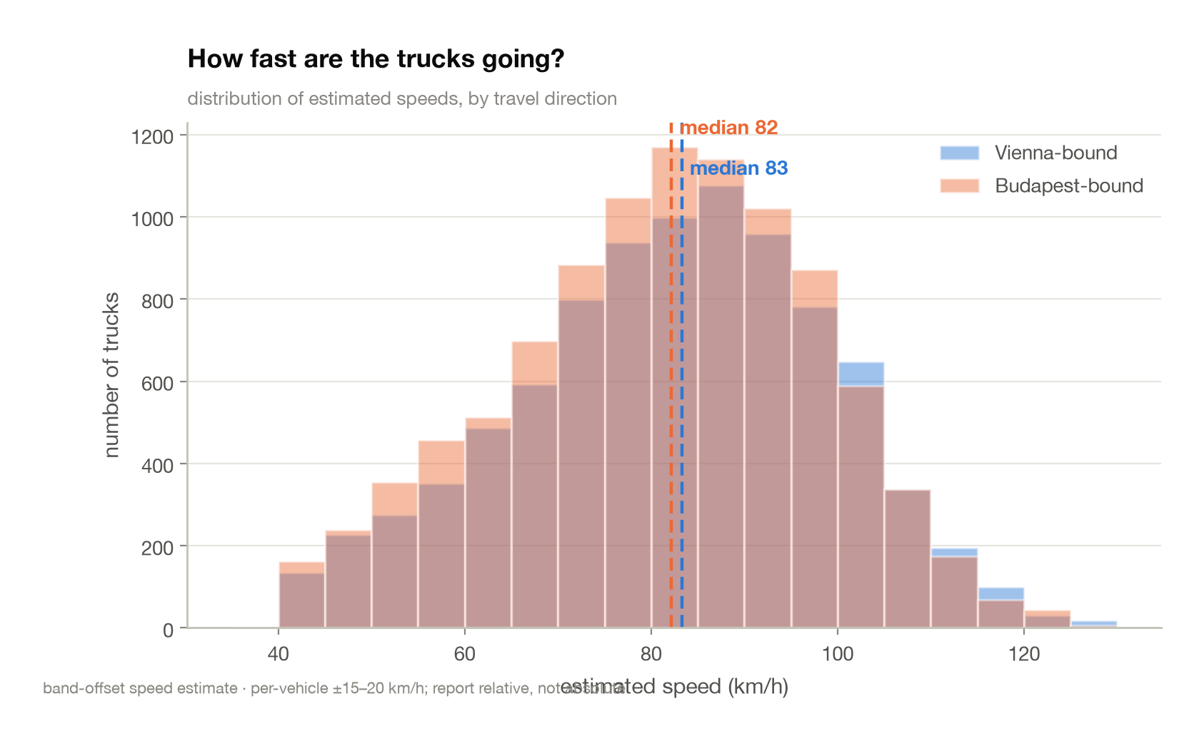
Truck speed along the Budapest–Vienna corridor — Median truck speed in each stretch of the route. Trucks run at a governed 80–90 km/h across most of the corridor, in both directions — but there’s a clear slow zone in the eastern third, where the median sags to the mid-60s.

The overall median comes out around 80 km/h, exactly where you’d expect EU-governed lorries to sit, and 86% of all detections land in the sensible 60–120 km/h band — a good sign the method is measuring real vehicles and not noise. That slow zone east of Tatabánya is real and repeatable. My first guess was terrain — the M1 climbs through some low hills there. That guess was wrong, and the satellite data itself proved it. Read on.

A construction project, caught in the act

On 1 September 2025, Hungary began its largest-ever motorway project: widening the M1 from 2×2 to 2×3 lanes along the 78 km from the M0 junction (Budapest) out to the Concó rest area near Komárom — precisely the eastern third of my corridor, and precisely where that slow zone sits. The dataset happens to straddle the start date, so I could compare the same stretch of road, in the same summer season, before and after the diggers arrived:

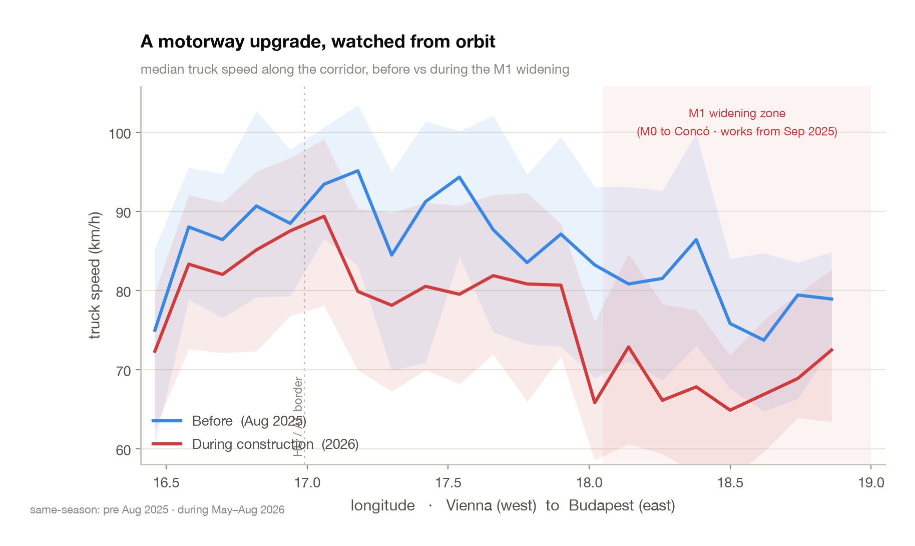
Truck speeds before and during the M1 widening — Before (August 2025) vs during (2026). West of the works the two lines sit on top of each other — nothing changed. Inside the widening zone, “during” drops well below “before”.

The numbers are unambiguous. In the work zone the median truck speed fell from about 80 km/h to 68 km/h, and in the worst-hit stretch around Tata it dropped from 86 km/h to 66 km/h — a 20 km/h collapse. Crucially, the untouched western corridor barely moved (a couple of km/h, within noise), so this isn’t a general slowdown or a quirk of the method — it’s localised exactly to the roadworks.

And it settles the earlier mystery: the slow spot is not the hills. The hills were there in August 2025 too, when trucks sailed through at 86 km/h. The 20 km/h drop only appears after construction started. So what looked like terrain was actually a construction project — one whose start date I could confirm from a press release, and whose footprint I could then watch unfold from space, weeks at a time. (The works run to 2028–29, so this slow zone will be a fixture of the data for years — and the western Concó–Hegyeshalom section, a separate later phase, should light up the same way when it begins.)

The weekend: a ban you can see from orbit

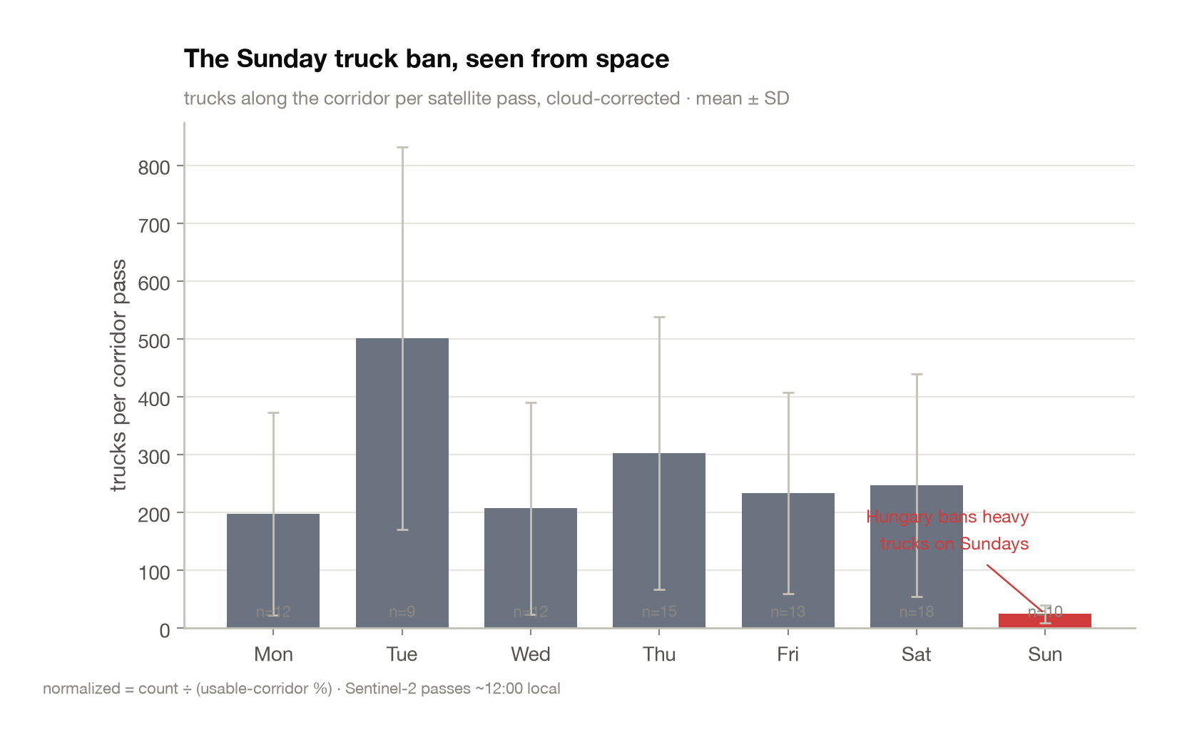
The Sunday truck ban, seen from space — Trucks counted along the corridor per satellite pass, corrected for cloud cover. Monday through Saturday look busy; Sunday almost empties out.

This is the single clearest signal in the whole dataset. Hungary — like most of Europe — bans heavy trucks (over 7.5 t) for essentially the whole of Sunday. Sentinel-2 flies over at around noon, right in the middle of the ban, and the count collapses to a small fraction of a weekday. You are, quite literally, watching a law being obeyed from 786 kilometres up.

Two countries, two rulebooks

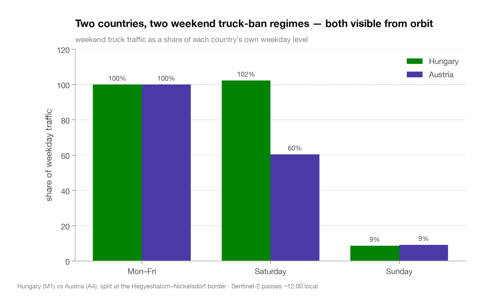
Two countries, two weekend truck-ban regimes — The same weekend, split at the border. Each country’s weekend traffic is shown as a share of its own weekday level, so the comparison isn’t skewed by the fact that the Hungarian stretch of road is longer than the Austrian one.

Because the corridor crosses a border, one image captures two different freight laws at once — and they look different. On Saturday at midday, Hungarian traffic is still at full strength (Hungary’s summer Saturday ban only kicks in at 15:00, after the satellite has passed — if anything traffic is slightly heavier, as hauliers push to finish before the weekend shutdown). Across the border, Austrian Saturday traffic is already suppressed to roughly 40% of its weekday level, reflecting Austria’s stricter weekend regime. Come Sunday, both countries fall to a near-total standstill. Two rulebooks, both legible from space.

Through the seasons

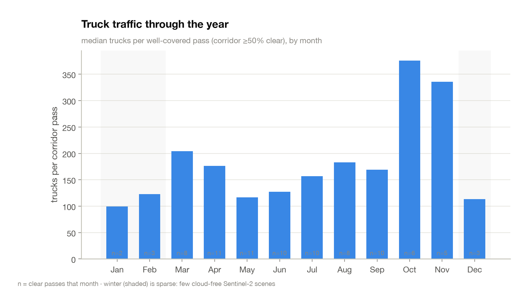
Truck traffic through the year — Median trucks per well-covered pass, by month. The low winter bars aren’t empty roads — they’re cloudy skies (central-European winters yield very few cloud-free Sentinel-2 passes over a 240 km corridor, the honest limit of optical monitoring). The higher autumn bars are consistent with the real freight calendar — a mid-summer lull around the August holidays and a pre-winter peak — but with only a handful of clear passes a month, and detection rates that shift a little with the seasonal sun angle, read the month-to-month heights as suggestive rather than exact.

The speed distribution

Distribution of truck speeds — How fast the trucks are going, split by direction. Both directions cluster tightly around the governed motorway speed, near-perfectly mirroring each other — a nice internal consistency check on the method.

6. Honest limitations

This is a genuinely useful measurement, but it is important to be clear about what it is not:

It counts a relative trend, not an exact total. Fisser’s own validation shows the method under-counts the true number of trucks (faint ones, trucks under thin cloud, or too close together are missed). The shape of the signal — more on weekdays, fewer on Sundays, a summer peak — is trustworthy; the absolute number on any single day is not.
One snapshot per pass, clear skies only. We get roughly one usable, cloud-free look every few days, always around noon. This says nothing about night traffic, rush hours, or overcast days. Winter, being cloudier, yields far fewer scenes.
Per-truck speed is rough — plus or minus 15–20 km/h for any individual vehicle — though averaging many trucks over a stretch of road tightens that up considerably.

None of this is a flaw in the approach; it’s the honest envelope of what free, 10-metre, twice-weekly imagery can tell you. Within that envelope, you can watch a nation’s freight rhythm — weekday rushes, weekend bans, holidays, seasons — from orbit, at no cost.

7. Satellites aren’t the only way — but they’re the great equaliser

To be clear: satellite imagery is not the best way to count traffic, and often not even a good one. If you run a road agency, you have loop sensors buried in the tarmac and cameras on the gantries. And if you want the richest picture of how vehicles actually move, you buy mobile-phone data — telecom operators and data brokers sell anonymised, aggregated location traces that yield continuous, 24-hour, all-weather traffic counts and full origin-to-destination flows. Compared to that, a satellite offers one cloud-free glance every few days, always around noon. For routine monitoring, phone data wins easily.

So why bother with satellites? Because of one property nothing else has: they cover everywhere, for everyone, on identical terms. The same free Sentinel-2 images every road in every country to the same standard. You need no deal with a local carrier, no data-sharing agreement, no vendor who happens to operate in that market — and crucially, it works where mobile-movement data simply isn’t for sale: smaller or poorer countries, places with strict privacy regimes or uncooperative authorities, border regions, conflict zones. On top of that, the decade-long archive lets you measure the past — you can study a country’s 2018 freight today, something no phone-data broker will sell you after the fact.

That’s the real case for this method. Not that it beats a traffic sensor on any single road, but that it lets you ask “how does freight move here?” for any place on Earth — including the many where nobody is selling the answer — on the same footing, from a public, free, and permanent record.

8. Resources & credits

The method (all credit to the originators):

Fisser, H., Khorsandi, E., Wegmann, M., & Baier, F. (2022). Detecting Moving Trucks on Roads Using Sentinel-2 Data. Remote Sensing 14(7), 1595.
Heiselberg, H. (2019). Aircraft and Ship Velocity Determination in Sentinel-2 Multispectral Images. Sensors 19(13), 2873.
Fisser’s original Sentinel-Hub “truck detection” custom script (the rule-based thresholds this implementation follows).

The data:

Accessed via the Element 84 Earth Search STAC API and the AWS Open Data sentinel-cogs bucket (no authentication required).
Mission facts (three satellites, ~786 km sun-synchronous orbit, ~10:30 local overpass, 13 spectral bands, ~5-day equatorial revisit over global land, decade-long archive): ESA Sentinel-2 mission documentation and the Sentinel-2 User Handbook (sentinels.copernicus.eu).
Inter-band time offsets: ESA Sentinel-2 MSI handbook; Binet, Bergsma & Poulain (2022), Accurate Sentinel-2 Inter-band Time Delays, ISPRS Annals.
Road geometry: OpenStreetMap contributors.
M1 widening schedule (start 1 Sep 2025, M0→Concó, 2×3 lanes): Magyar Építők and MKFE (Hungarian Road Haulers’ Association) reporting; live restrictions at development.mkif.hu/m1.
Weekend/holiday HGV driving bans (Hungary: Sundays and public holidays, with a summer Saturday-afternoon ban; Austria: Saturdays from 15:00 and all of Sunday/holidays, plus a nightly ban): the respective national road-traffic regulations.

The tools: Python, with rasterio / rioxarray (imagery), pystac-client (search), geopandas / shapely / osmnx (geometry), numpy / scipy (detection), and matplotlib (charts). Everything runs on a laptop.

Code, the scene manifest, and the full detections table are in the project repository; a curated sample of the source imagery (127 MB) is archived with the tagged release.